Satellite Images Object Detection: 95% Accuracy in a Few Lines of Code
The question is not ‘If’, but ‘how’ image-based insights should be consumed. Exploit business opportunities with satellite data.
Tuesday, 4 February, 2020
Satellite Images Object Detection: 95% Accuracy in a Few Lines of Code
Ship Surveillance & Tracking with TensorFlow 2.0: The Basic Solution
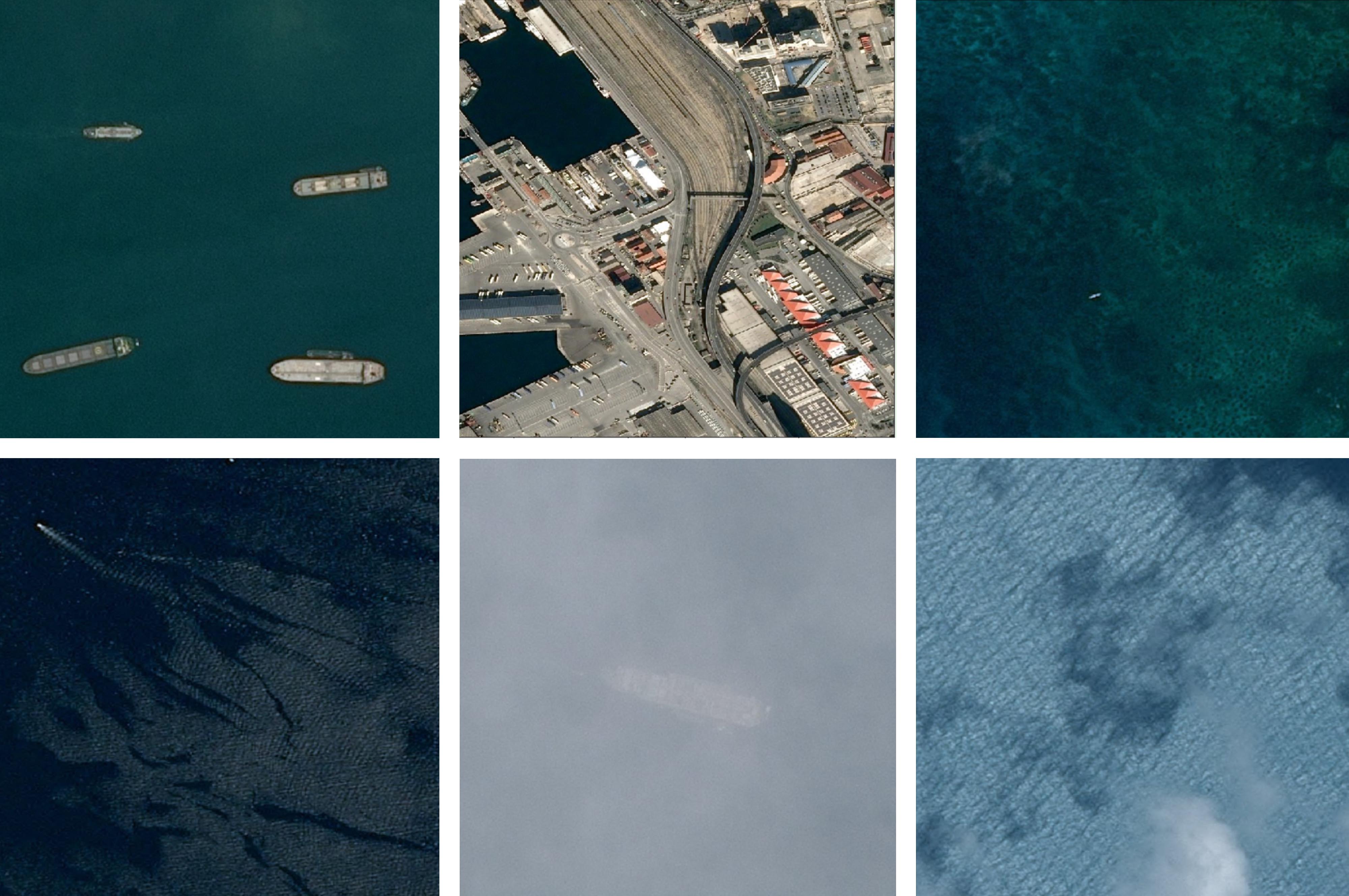
Diversity of satellite images conditions and scales makes object detection one step harder
The Question Is Not “If”, but “How” Image-Based Insights Should Be Consumed
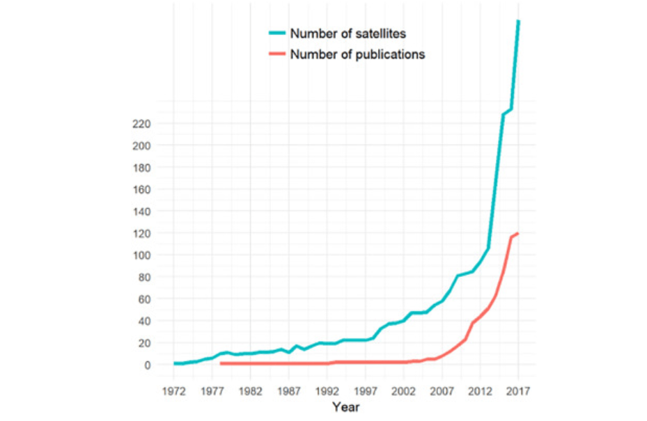
Given the exponential growth of images, and in particular optical, infrared and SAR satellite images, business opportunities are growing faster than the number of data scientists that know how to handle them.
For companies used to consume structured data, this means:
- Dedicating a number of their data scientists to develop image processing skills in-house, or
- Consuming already processed feeds, for example Vortexa and its SDK or its datasets on AWS data exchange in the case of ship analytics.
Target audience for this post:
- The data scientist tasked with developing image processing skills will be interested in the simple implementation of Part 1, as well as the thinking process in dealing with the often unspoken architecture and optimisation choices made in Part 2.
- The reader interested in consuming already processed feeds might want to look at images and their captions in both posts, and get a feel for what’s involved in object detection, and their interpretability.
This is the 1st part of a 3 blog posts series:
- Ship detection – Part 1: ship detection, i.e. binary prediction of whether there is at least 1 ship, or not. Part 1 is a simple solution showing great results in a few lines of code
- Ship detection – Part 2: ship detection with transfer learning and decision interpretability through GAP/GMP’s implicit localisation properties
- Ship localisation – Part 3: identify where ship are within the image, and highlight with a mask or a bounding box
What you will learn in this post (Ship detection – Part 1):
- Context: satellite imaging context & opportunities
- On the fly preprocessing generators with Tensorflow
- Learning rate selection technique
- Simple ConvDenseNet (LeCun style) implementation, reaching 95% accuracy while having seen the data set only 2.5 times
Context, Motivation and Opportunities
With the increase of satellites in orbit, daily pictures of most of the world are now widely available. Data sources include both free (USGS, Landviewer, ESA’s Copernicus etc) and commercial (Planet, Orbital insight, Descartes Labs, URSA etc) entities. The competition is fierce, and seems to yield very fast innovation, with companies such as Capella Space now pitching hourly updates by launching constellations of small satellites of only a few kg. Those satellites increasingly cover beyond the optical visible spectrum, notably Synthetic Aperture Radar (SAR) which offer the benefit to work independently of clouds or daylight. Along with the growth of other image sources, the ability to interpret image data is a key to untapped commercial opportunities.
The monitoring of human activity is increasing for the purpose of fishing, drilling, exploration, cargo and passenger transport, tourism, for both governmental and commercial purposes, particularly at sea. For ship tracking in particular, satellite images offer a rich complement to baseline cooperative tracking systems such as AIS, LRIT and VMS.
Feeding the Beast: Pre-processing Steps
- Label each image as ship / no-ship.
- Mini-batch data into 40 images chunks. Using batches > 1 leverages vectorisation and makes computation faster compared to stochastic gradient descent (i.e. batch size = 1). Using smaller batches (~20-500) than the entire dataset (200k images here) first allows the data to fit in memory, and the extra noise tends to prevent premature convergence on local minima.
- Reduce the image size from 768 x 768 x 3 to e.g. 256 x 256 x 3, to make training faster, and reduce overfitting. Using modern ConvNet (fully convolutional or with GAP/GMP), it is good practice to start training with small images and fine tune with larger images later.
- Data augmentation: flip horizontally and vertically initially. Extra distortions could be added later on, when the model starts overfitting to squeeze extra performance.
- Renormalise magnitude from [0, 255] to [0, 1].
Here is how we conduct this pre-processing on the fly with Keras’ ImageDataGenerator class, with the labeling done with flow_from_dataframe, all feeding later on into the fit / fit_generator API:
1st Architecture – A Simple ConvDense Network
Starting simple and iterating:
- Images are represented as 4 dimensional tensors: batch size, height, width and channels (RGB at the input, layers of features deeper in the network)
- 3 blocks of convolutional + max pooling to extract features from the image (with 3×3 sliding windows). As we go deeper into the network and work with increasingly abstract features, the image dimension is reduced (256 -> 128 -> 64 -> 32) while the number of channels is increased (3 -> 16 -> 32 -> 64)
- 1 dropout layer for regularisation (i.e. prevent over-fitting)
- 2 dense layers to make sense of all these extracted features, and combine the presence or absence of those to decide whether there is a ship on the image or not
To optimise this model we need:
- loss: sparse_categorical_crossentropy if using softmax as the last activation, or as there are only two categories binary_crossentropy with sigmoid as the last activation (can also work with raw logit, with a twist, see Part 2)
- optimiser: one choice is using Adam, and tune (image below) or cycle the learning rate (to get out of local minima, more on this in Part 2). For this first run I ended up choosing a learning rate of 3E-4. The other parameters controlling the exponentially weighted averaged moments of gradient use the default values (first order is called momentum and parameter beta1, second order is called RMS prop and parameter beta2).
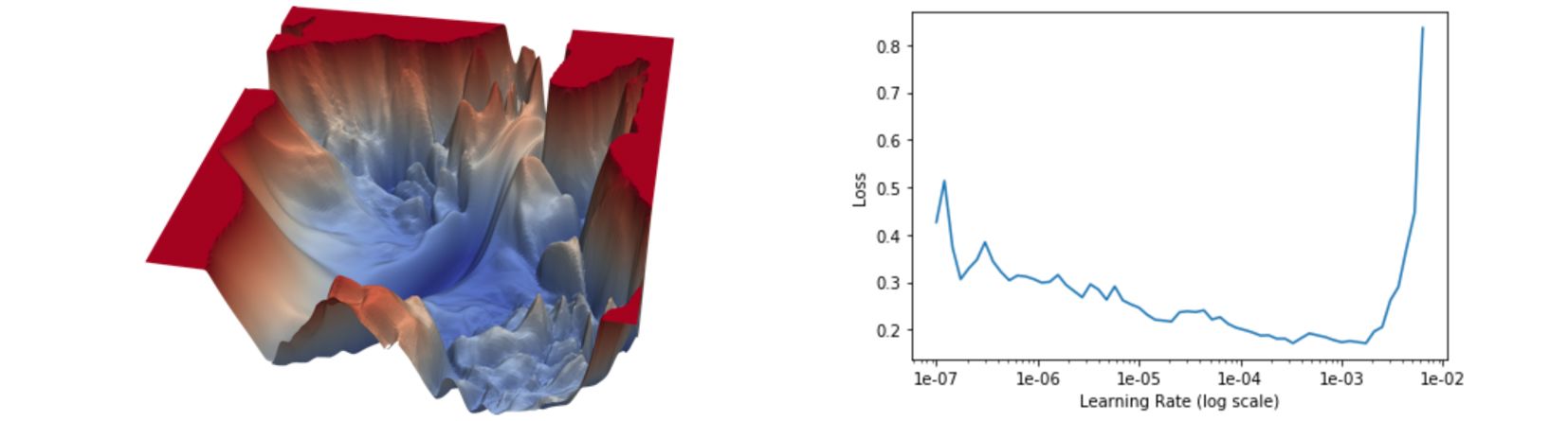
[Left] Illustration of a neural network optimisation problem: the goal here is to find the minimum while being blindfolded. [Right] Exploring the learning rate landscape – we want to pick the learning rates with the largest loss gradient, and stay away from divergence. Method: start at a very low LR, say 1E-7, and at each batch increase the LR slowly, until a high LR, say 1E-2 or even 10. This is a very approximate method, as both weights and data are changing as the learning rate increase. However, this is computationally cheaper than running multiple simulations in parallel, so hopefully a reasonable stop-gap solution to pick a safe learning rate.
Here is the Tensorflow 2.0 implementation:
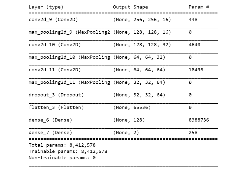
Keras’ architecture summary of the network described earlier, following a classic LeNet design (LeCun) of a series of convolutional and max pooling layers, followed by dense layers. Note that most of the weights are in the dense layer, despite limiting the image size to 256 x 256 pixels. More recent architectures have moved away from this design, and are now fully convolutional, avoiding this concentration of weights on a single layer, which, all things being equal, tends to overfit and yield lower performance.
Here is the basic Tensorflow / Keras code to train the model, with the parameters used:
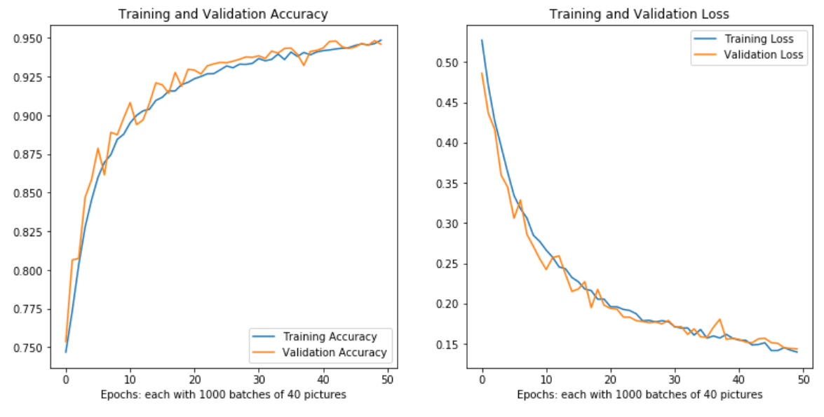
By showing this simple neural network our training set about 2.5 times, we reached 94.8% cross-validation accuracy. A naive approach given the class imbalance would be 77.5%.
Note that the model is still learning, and that we aren’t yet observing signs of overfitting. This is by design, due to the relatively small size of the model compared to the dataset size (200k + 600k augmentation), and the dropout layer.
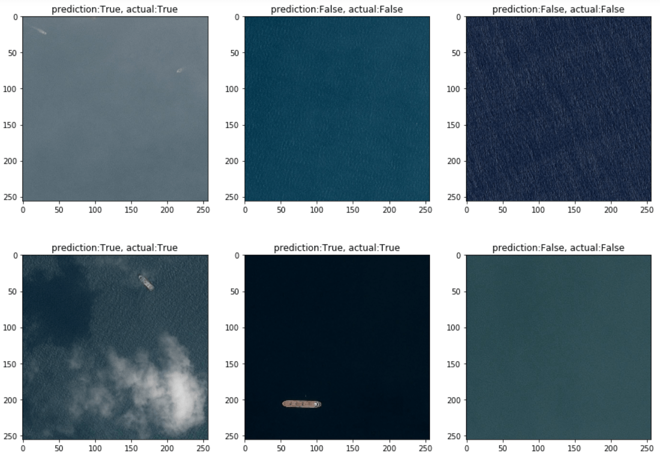
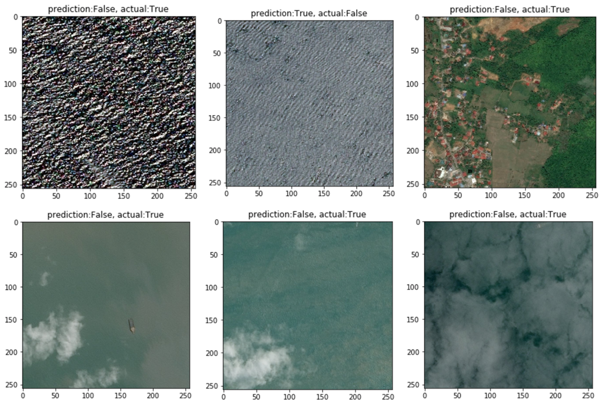
Examples of misclassification below. We can see that some cases are hard to resolve to the human eye while there still seems to be a minority of easy wins. Also interesting that a fraction of labels seem wrong: another reason to avoid overfitting.
Improving This Model
A tested improvement to this model is to add batch normalisation between weights and activation: it allows the model to reach 93% accuracy in only 10 pseudo-epochs, compared to 25 pseudo-epochs without. The plateau seems the same, close to 95% (only trained 40 pseudo-epochs).
Further improvements could involve more capacity for our model as it may underfit slightly currently, as well as exploit higher resolution images.
An issue with this architecture is that input image size is fixed. That can be solved through
- Global Averaging / Max Pooling layers (GAP / GMP) at the end, just before a or multiple dense layers, for a global aggregation over the spatial dimensions (batch size, height, width, channels) -> (batch size, 1, 1, channels), irrespective of image size.
- Fully Convolutional Network (FCN), using a similar idea but generalising it with a learned spatial operation through a 1×1 depth filter.
In the second part of this post, we explore the former architecture, along with a deeper network.
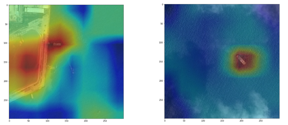
Visualisation of the model’s attention, and with it emerging localisation properties, while having never labeled ship location! Explanation in part 2 of this post.
Author: Romain Guion, Head of Signal Processing and Enrichment
For more practical tips on Data Science and Tech – follow the VorTECHsa team on Medium


