What’s the point (in polygon)?
Sometimes writing your own algorithm out-performs a library by 3 orders of magnitude.
Written by Ed Wright, Vortexa Lead Geospatial Engineer
Who should read this article: engineers, data scientists, people interested in mathematics, or geospatial engineering
We probably all came across polygons at school. Right-angled triangles and fun with Pythagoras’ theorem, hexagons, isosceles trapeziums. I’ve never really had a use for an isosceles trapezium, though I saw a spectacular one once by Christo and Jean-Claude in the Serpentine. These shapes are with us everywhere, whether in the shapes forming circuits within the silicon chips in your smartphone, to geofences you set up when asking for a reminder in a certain place, to the planning of cities and residential zones. Everywhere.
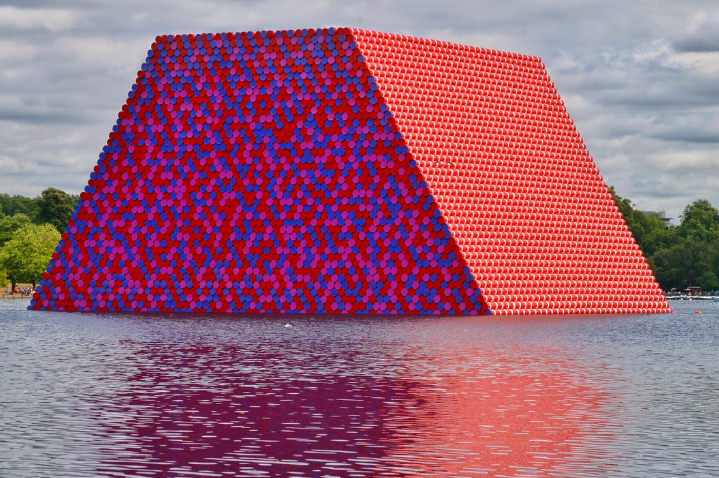
Christo and Jeanne-Claude: The London Mastaba, photo by Gary Etchell
Polygons can impart design, can subdivide resources, and can impart meaning. If I share my location with my partner, and she sees I am at home (in that small shape on a map which we call home, essentially a polygon though we’d never call it that), crossing that location, that point, with that shape, has meaning. This example is a visual representation of a simple mathematical problem called point-in-polygon. How to determine whether a point is within a shape.
We have quite a lot of polygons at Vortexa too, and we infer a lot of meaning from them.
We break our world down into macro-scale regions such as countries, into ports where ships can visit, and into numerous other categories which have a business and/or technical meaning for the problems Vortexa has set out to solve. Indeed, almost all of the Earth which is not covered by permanent ice, is covered by Vortexa polygons.
So here’s an engineering problem we had to address:
- We have a lot of polygons (thousands), many of them very complex
- We monitor a lot of ships (we call them vessels)
- We have a lot of signals from those ships (billions)
- The goal – work out who went where, when
If you’re anything like me, when you see a problem which has “a lot” in it three times or more, it sounds like there is some fun to be had.
Basics
The purpose of this post is not to explain the basic polygon math, that can be found in many places including Wikipedia. Besides, what is the first (responsible) thing a good software engineer would do? Find a well maintained library which does the job for us.
For many reasons beyond the scope of this article, Java was the tool of choice for this task, and the excellent Java Topology Suite (JTS) ticks the box for many geometrical operations. It is a Swiss-Army-knife of a library. Great, no wheels re-invented here! If Java is not your tool of choice, read-on for the techniques discussed here are language agnostic.
“…Indeed, almost all of the Earth which is not covered by permanent ice, is covered by Vortexa polygons.”
What we’re trying to do is loop through signals from vessels. These signals contain timestamps and coordinates, latitude/longitude data from GPS receivers. For each signal, we compare it with our polygons, and record which polygons we have entered and which we have left. Every vessel in our system thus becomes a little state machine:

Hold on a sec
So we have thousands of polygons. Billions of signals. [sound of a pen scribbling on an envelope] That means trillions of calculations. We can scale by sharding the problem by vessel, using threads and scaling horizontally by throwing hardware at it, but isn’t this going to get expensive quickly? What if we need to iterate on the software design, or the polygon geometry, or both?
To save you the trouble, I did some benchmarks with our test polygons and about a million vessel signals. This test set and hardware are going to remain fixed as we progress. The absolute figures do not matter so much, but we’ll use them for comparison. The benchmark is counting point-in-polygon hits but doesn’t have the visit-started, visit-ended logic alluded to above.
Using four cores, sharding by vessel and using threads, but doing a naïve call to the JTS Geometry.contains(Geometry) method takes 2621 seconds to run.
Clearly running this against billions of signals is going to be expensive, not-fun or both.
What is my library doing?
The short answer is: a great deal.
One of the strengths of JTS is also a weakness. It is a super sophisticated, generic library. You want to use various coordinate systems? Sure. 2D or 3D shapes? No problem. Advanced comparison and union operations? Easy. The list goes on and on.
Even the contains() method is comparing two geometries. These could be 3D shapes and the library can calculate whether one is fully contained within the other. This is going way beyond our needs of a point in a 2D polygon.
What this does mean though is a simple call to contains() is actually doing a whole bunch of work. Stepping into the source (I do recommend learning what the libraries you use actually do) in a debugger shows many layers of complexity, deep stack traces, which is appropriate given the generic nature of the library.
Step One – avoid calling JTS if necessary
The easiest way to avoid the overhead of calling all that JTS logic is? to not call it. How can we do that?
Bounding boxes.

Here I have a fluffy cloud polygon (it’d look angular under a microscope, trust me), and I’ve surrounded it by a bounding box.
So now my new improved algorithm can store a bounding box for every polygon against the polygon, and do a really cheap range check on the coordinates to find easy cases where we’re sure the point is not in the polygon. If it’s not in the box, it’s not in the polygon. This is not perfect, if the point is within the box but outside of the polygon we still need to do the math (call JTS) to find out – but statistically we’ll need to do it less.
Benchmark result: 2443 seconds.
Step Two – Avoid JTS
The approach here is to create a Java class to represent a polygon with latitude and longitude in two double[] arrays. The ray casting algorithm mentioned earlier is implemented. The actual implementation handles cases such as multi-polygons and polygons with holes in them. The code also includes a bounding box filter like the previous test.
So now we have our own home-grown point-in-polygon math, is it worth it?
Benchmark result: 125s
This is 21x faster than using JTS.
Step Three – part 1, R-Trees
A huge inefficiency we have here is for every signal, we’re still testing every polygon. How can we do an efficient lookup of polygons near the point we wish to test, discounting all those far away which we know don’t count?
One answer could be using a geospatial lookup structure such as an R-Tree. These act a little like maps or dictionaries, except the semantics are:
“Given a coordinate, give me all entries (or the nearest) within a certain radius”
The internal structure of the R-Tree means such queries can be answered efficiently.
The problem we encountered at Vortexa is our polygons vary wildly in size, from terminals within a port to the size of countries like Russia. Clearly if we index our polygons by their centroid, the search radius needs to be vast (so we can find Russia when we want to) but this means we’ll also pull in lots of smaller polygons from far away.
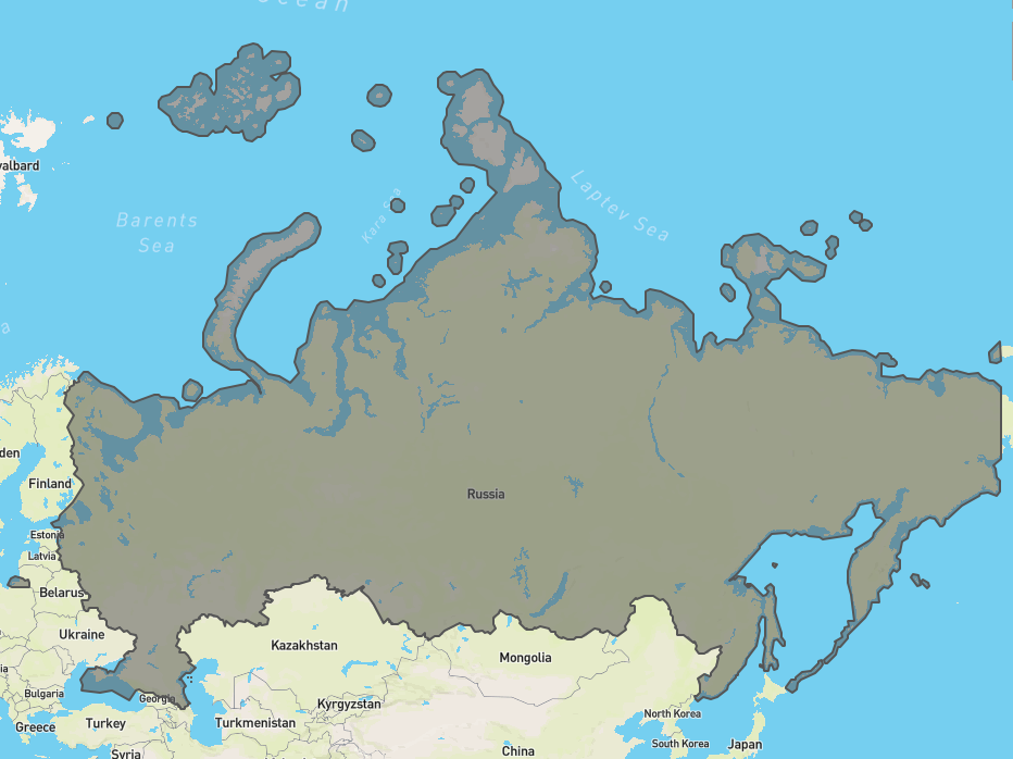
Technically, the radius would need to be at least the distance from Russia’s furthest extremity to Russia’s centroid. It’ll be very inefficient.
So, an alternative is to “paint” the larger polygons with regularly spaced points (where they fall within the polygon), and index those in the R-Tree. We’d also need to add the centroids of each component part, so we can capture smaller parts of this complex multi-polygon.
If we (say) placed points every 200km, then we could search the R-Tree with the smaller radius of approximately 142km (remember Pythagoras? The hypotenuse of a right-angled triangle with 100km sides). Or we could choose a smaller figure.
This approach was tried at Vortexa in the past, and worked, but we found a better way.
Step Three – part 2, a grid
The R-Tree alternative, while not mathematically balanced or sophisticated, is simple. Sometimes, with O(N) or O(log N), the N matters!
Let’s split the world up into a grid, and for each square, list which polygons are present there – we pre-calculate this and store it.
When we come to process, from a signal we find the square very quickly, and then we have a much smaller shortlist of polygons to process. We chose degree squares, which divides the planet into 64,000 squares. This data structure is not balanced like an R-Tree, but it is simple and thus super fast.
Benchmark now gives us: 8023ms
We are now 327x faster than the initial approach. Job done?
Step Four, back to the math
All the calculations to date have been using 64-bit floating point math. The fractional part (the mantissa) is 52-bits. Given our largest (in magnitude) coordinate value is +-180º, that gives us an accuracy of 180 / 2^52 ~= 4 x 10-14 degrees, which given we have approximately 110km per degree at the equator, works out at about 4.4nm. I’m sure you’d agree we don’t need to track vessels moving across the high seas to nanometer precision. Not to mention GPS error margins.
Can we use 32-bit floats?
Here we’d only have 23-bits to play with, so
180º / 2^23 * 110000 ~= 2.36m of precision
This could be ok.
However, modern CPUs, although they have powerful floating-point hardware, are always significantly faster at integer math. If we were to store coordinates as integers, scaled to a positive 31-bit range (remember we’re using Java? Integers are signed and we don’t want those complications in our math), how would that look?
360º / 2^31 x 110000 ~= approx 2cm
Note we have no mantissa concerns this time so we calculate based on the whole range of longitude, 360º.
So to avoid mixing things up, let’s re-run the test we did in step 2, using integers. As a bonus, we can pack both latitude and longitude values into 64-bit words and use one long[] array instead of two int[] arrays. Locality of reference when accessing memory is our friend. Shift and masking operators are fast.
Repeating step two as a control (just bounding box test and new geometry math), our benchmark result is 75s.
This is 1.67x faster than using double-based custom polygons.
Folding in the grid lookup back in, we get a benchmark result: 7876ms
The improvement factor compared with step three is less, because with the grid lookup proportionally less time is spent within the geometry math code.
We are now 333x times faster than the initial no-frills use-the-library approach. I don’t believe in 10%.
Step Five
We didn’t rest there. There’s another technique we’ve employed, which boosted performance another 8x faster still, bringing us 2655x faster than naîve JTS usage. No cheating, this is sticking with Java and measuring using the same data / hardware and producing the same results.
To find out how we did it at Vortexa, look at our open positions and get in touch.
Conclusions
|
Technique |
Absolute time |
Speedup factor |
|
Pure JTS |
2621s |
1.0 (reference) |
|
Bounding-box check + JTS |
2443s |
1.07 |
|
Custom double based polygons |
125s |
21 |
|
Custom int based polygons |
75s |
34.9 |
|
Grid technique with double polygons |
8023ms |
327 |
|
Grid technique with integer polygons |
7876ms |
333 |
|
Step Five |
987ms |
2655 |
The game-changing optimizations were:
- Replacing JTS math with custom integer based math (about 30 lines of code in reality)
- Using a square-degree based grid for polygon lookup, avoiding math on polygons which do not concern us
Optimizations are not the first (or second) things we should consider when writing code. Projects need to be maintained by the whole team, including team members who may join after you’ve moved onto something else. Clarity, maintainability and test-coverage are paramount.
However, sometimes you may find a hotspot where pushing harder is worth it. In this article we’ve been saving minutes, but in reality at Vortexa we regularly process five or six orders of magnitude more data. Factors such as lead time to production or iteration speed do matter.
So with this, in production we have some heavily unit-tested and regression-tested, well documented “extra” code (a library can indeed do the work) but have achieved a 2655x processing efficiency boost. The savings in compute time and human time (getting results early, iterating) are real. The code has proven stable and is not a maintenance burden.
I hope you have enjoyed this journey.
Vortexa
I’ve been with the company since the very first day and seen it grow and flourish. My motto here is “Never bored”. There is so much to do, so many fascinating problems to solve and the chance to make a real difference with customers, growing personally in the process.
We are continually looking for new talent, be that software engineers (Python, Java, Kotlin, Scala, Rust and other languages), data scientists, devops specialists, analysts and more. See our careers page.


